Why Two Identical RO Plants Consume Different Amounts of Energy
Introduction
Two SWRO trains, same manufacturer, same membrane model, same array configuration, same design capacity — and at the end of the month, one plant is running at 3.8 kWh/m³ and the other at 3.2 kWh/m³. Same nameplate, an 18% gap in specific energy consumption (SEC). This is not a hypothetical; it is a recurring finding in third-party performance audits across the GCC, and benchmarking work published by organizations such as the International Desalination Association and Global Water Intelligence has repeatedly shown the same pattern industry-wide: plants of near-identical design routinely show wide SEC variance once they’ve been in operation for more than a year.
Design documents describe a plant on paper. SEC is determined by how that plant is actually operated, maintained, and instrumented — variables a P&ID cannot capture. For plant managers and process engineers, the gap between “as-designed” and “as-operated” energy performance is where real operating cost lives, and where the largest RO energy optimization opportunity exists without a single capital upgrade.
This article breaks down why nominally identical RO plants diverge in energy consumption, which variables get overlooked in routine reporting, and what an operations team can act on this quarter to close the gap.
Key Takeaway: SEC divergence between identical plants is very rarely one dominant cause. It is the sum of five or six individually small deviations — each worth 0.05–0.3 kWh/m³ — that compound because none of them trip an alarm on their own.
Why Identical RO Plants Don’t Consume the Same Energy
Two plants built from the same design package rarely stay identical past commissioning. The moment a plant starts producing water, dozens of small deviations begin compounding.
Design Philosophy vs. Operating Reality
A design package specifies a target flux, recovery rate, and feed pressure at a single design point — usually nominal seawater conditions (commonly 35 g/L TDS, 25°C for Red Sea/Gulf-adjacent design bases, though local intake salinity varies materially by site). Actual feed salinity, temperature, and seasonal variability rarely sit at that design point for more than a few weeks a year.
Feed water temperature has a direct, quantifiable effect on membrane permeability: as a working approximation, membrane water permeability increases roughly 3% per °C rise in feed temperature (the temperature correction factor, or TCF, referenced in ASTM D4516 normalization practice). A plant seeing a 10°C seasonal swing — not unusual between Gulf winter and summer intake temperatures — will see membrane permeability shift by roughly 30% across the year if feed pressure setpoints aren’t re-tuned seasonally. A plant operated rigidly against original design setpoints, rather than re-tuned against real seasonal conditions, will consistently over-pressurize in winter (wasting pumping energy against a membrane that’s now more permeable than the design basis assumed) or under-recover in summer.
Operating Strategy
Some operations teams run trains at fixed setpoints regardless of feed conditions; others actively re-optimize recovery and flux against real-time water quality and energy cost. The second approach consistently produces lower SEC, because feed pressure is being spent only where it is needed rather than held at a conservative margin around the clock. In practice, this is the difference between a control philosophy built around static setpoints locked at commissioning and one built around continuous re-optimization — a distinction that shows up repeatedly in third-party plant audits as the single largest operating-discipline gap between top-quartile and average-quartile plants.
Hydraulics
Piping layout, valve positions, instrument tie-in points, and the physical distance between the high-pressure pump and the membrane vessels affect head loss. Two “identical” plants built on different sites, with different pipe runs and fitting counts, will have measurably different hydraulic losses — even before accounting for wear. A single additional 90° elbow and a longer suction run can add a meaningful fraction of a bar in avoidable head loss; multiplied across a full train’s flow rate, this is a fixed energy tax that exists purely because of layout, independent of process performance.
Recovery Rate
Recovery rate has a nonlinear relationship with energy demand, and the mechanism is straightforward mass balance: as water is recovered as permeate, the salt rejected by the membrane concentrates in a shrinking reject stream. For a feed TDS of 35 g/L, concentrate TDS scales approximately as TDS_feed ÷ (1 − recovery fraction):
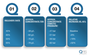
Using the van’t Hoff approximation π ≈ i·C·R·T, simplified to roughly 0.8 bar per g/L TDS at 25°C for a seawater ionic mix — illustrative, not a substitute for full mass-transfer modeling, which must also account for concentration polarization and the net driving pressure needed to hold target flux.
The practical consequence: pushing recovery from 45% to 50% doesn’t cost “a bit more energy” — it raises the osmotic pressure the pump has to overcome at the tail end of the array by roughly 10%, which is exactly why plants pushed to a higher recovery than their feed chemistry comfortably supports show disproportionate SEC increases and elevated scaling risk simultaneously. The two symptoms share a root cause.
Fouling
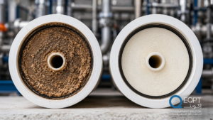
Fouling increases differential pressure (ΔP) across the vessel and forces the pump to work harder to sustain design flux. A train fouling faster than its counterpart — due to pretreatment performance, seasonal algal blooms, or inconsistent chemical dosing — will silently drift toward higher SEC weeks before anyone flags it on a maintenance report.
Engineering Note — Fouling Is Not One Mechanism:
“Fouling” gets used as a catch-all term, but colloidal fouling (particulate/organic deposition, addressed by improved pretreatment and coagulation), biofouling (microbial biofilm growth, addressed by biocide dosing and nutrient control), and scaling (mineral precipitation, addressed by antiscalant dosing and recovery control) have different root causes and different corrective actions. Applying a scale-focused CIP (low-pH, acid-based) to a biofouling problem, or vice versa, produces temporary ΔP improvement followed by fast recurrence — a pattern experienced operators use as a diagnostic signal that the wrong cleaning chemistry was applied, not that cleaning failed outright.
Pressure Losses
Every strainer, cartridge filter, elbow, and control valve represents a pressure drop that the high-pressure pump must compensate for. Partially clogged cartridge filters or an undersized bypass line can add measurable pressure loss that never appears as a discrete line item — it just appears as a slightly higher pump discharge pressure that operators assume is “normal.” A cartridge filter approaching its rated ΔP limit (typically replaced at 1.0–1.5 bar differential depending on OEM guidance) that’s instead run to 2 bar because replacement was deferred is, in effect, an unbudgeted pumping energy penalty hiding inside a maintenance deferral decision.
Membrane Selection
Not all membranes rated for the same application perform identically. Differences in permeability, rejection characteristics, and fouling resistance between membrane batches — even within the same product line — translate directly into different feed pressure requirements to hit the same permeate flow and quality targets. This is why membrane replacement decisions should be evaluated against normalized permeate flow and salt passage data, not simply against membrane age or a fixed replacement interval.
Hidden Factors Affecting Energy Consumption
Beyond the structural factors above, there is a second layer of variables that rarely appear in a design review but consistently show up in an energy audit.
Feed Water Quality
Seasonal shifts in temperature, salinity, turbidity, and organic loading change the osmotic pressure and fouling potential of the feed. A plant intake near a shipping channel, industrial discharge, or seasonal algal bloom zone will see feed water quality swings that a plant with a cleaner intake never experiences — even if both plants are rated for “seawater” conditions on paper.
Pump Efficiency
High-pressure pumps lose efficiency over time due to wear ring clearance, impeller erosion, and bearing wear. A pump operating 5–8 percentage points below its original efficiency curve — common after several years without an overhaul — quietly increases specific energy consumption without triggering any alarm, because flow and pressure targets are still being met.
To put a number on it: a 5-percentage-point drop in centrifugal pump efficiency (e.g., from a design point of 80% down to 75%) typically increases SEC by roughly 0.15–0.25 kWh/m³, depending on the plant’s baseline SEC and the fraction of total power drawn by high-pressure pumping relative to ERD recovery. Across a 20,000 m³/day train running continuously, that’s on the order of 1,100–1,800 kWh per day lost to a degradation that never appears on a single alarm.
Engineering Note — NPSH and the Efficiency-Erosion Cycle:
Insufficient suction conditions relative to the pump’s required NPSH (NPSHr) cause cavitation, and cavitation erosion pits the impeller — which further degrades hydraulic efficiency and lowers the pump’s effective NPSHr margin over time, accelerating the cycle. Available NPSH (NPSHa) should be verified against the current NPSHr curve — not just the original commissioning curve — whenever suction-side strainer ΔP or feed tank level operating range has changed since commissioning. Pumps running consistently below their best efficiency point (BEP), typically outside roughly 70–120% of BEP flow, are also more prone to radial thrust-induced bearing wear, which shows up later as the same gradual efficiency loss.
Energy Recovery Devices (ERDs)
The ERD is often the single largest differentiator in SWRO energy performance. Isobaric pressure exchangers typically recover energy from the reject stream at 95%+ volumetric and hydraulic efficiency, versus 85–90% for older Pelton-wheel-based turbochargers. Moving from an 85%-efficient turbocharger to a well-maintained isobaric PX can reduce net SEC by roughly 0.4–0.8 kWh/m³ in a typical seawater application, depending on recovery rate and reject flow fraction — often the largest single lever in the entire energy balance.
The efficiency figure isn’t static, either. Isobaric PX units lose volumetric efficiency as internal seals wear and as small amounts of mixing occur between the high- and low-pressure streams inside the exchanger. A plant running an ERD at a reduced efficiency point — due to internal wear, incorrect flow balancing between trains, or improper commissioning — can lose several tenths of a kWh/m³ compared to a properly tuned unit of the identical model, and this degradation is invisible on a standard SCADA power trend unless ERD efficiency is tracked as its own KPI, separate from overall plant SEC.
Instrument Calibration
Pressure transmitters, flow meters, and conductivity analyzers that drift out of calibration lead operators to make control decisions based on inaccurate data. Typical high-pressure transmitters carry a stated accuracy of ±0.1–0.25% of full scale; on a 100 bar span, that’s a design tolerance of roughly ±0.1–0.25 bar. A transmitter reading 0.5 bar low is therefore already running at 2–5x its rated uncertainty — a sign it is overdue for verification against a reference standard (e.g., a portable deadweight tester or a calibrated master gauge), not just a routine drift.
That 0.5 bar error causes the control loop to push the pump slightly harder than necessary to “meet” a setpoint that is already satisfied — a small error that compounds into real energy cost over a full year of continuous operation. The same logic applies to flow meters: a magnetic flowmeter reading even 1–2% off true flow will distort every normalized SEC and recovery calculation derived from it, which means a plant can be measuring its way into a false sense of good performance.
Pretreatment Performance
Pretreatment quality directly dictates how much cleaning, backwashing, and chemical dosing the downstream RO system requires. A pretreatment train running marginally out of spec — slightly higher turbidity carryover, inconsistent coagulant dosing, or an underperforming media filter — forces the RO system to compensate through higher fouling rates and more frequent CIP cycles, both of which increase energy intensity (via train downtime, backwash pumping, and the cumulative flux loss each CIP cycle leaves behind even after cleaning).
Chemical Dosing Accuracy
Over-dosing antiscalant wastes chemical cost without improving performance; under-dosing accelerates scaling and increases differential pressure. Dosing pumps that aren’t periodically verified against actual flow rates — rather than assumed design flow — are a common, invisible source of performance drift in mid-sized plants, and this ties directly back to the instrument calibration issue above: a dosing pump calibrated against a flow signal that’s itself off by 2% is dosing incorrectly by roughly the same margin, silently, indefinitely.
Operational Optimization
Closing the gap between two “identical” plants is primarily a data and discipline problem, not a re-engineering problem.
Monitoring the Right KPIs
Total power draw tells you almost nothing on its own. The KPIs that actually diagnose RO plant health are:
- Specific Energy Consumption (SEC) — kWh per cubic meter of permeate, normalized for feed salinity and temperature (per ASTM D4516-style normalization practice)
- Normalized differential pressure across each pressure vessel and train
- Normalized permeate flow and salt passage, corrected to a reference temperature and pressure
- ERD efficiency, tracked independently from overall system SEC
- Pump efficiency, benchmarked against OEM curves at current operating points, not nameplate conditions
Best Practice Box — Normalizing SEC Correctly: Raw SEC (kWh/m³ = pump electrical input ÷ permeate flow) is only meaningful once corrected for feed temperature and salinity; otherwise a plant will appear to “improve” every winter and “degrade” every summer purely from the TCF effect described earlier, masking real equipment-level drift. Normalize before benchmarking month to month or train to train — comparing raw SEC across a seasonal boundary produces false conclusions almost every time.
Specific Energy Consumption as a Diagnostic Tool
SEC should never be tracked as a single monthly average. Trended daily and normalized against feed water temperature and salinity, SEC becomes an early-warning indicator — a slow upward drift in normalized SEC almost always precedes a visible fouling or mechanical issue by weeks.
Data Analytics
Plants generating years of SCADA historian data are almost always under-using it. Trend analysis across recovery rate, ΔP, SEC, and cleaning frequency reveals patterns — such as a recurring seasonal SEC spike tied to a specific water quality window — that a monthly performance report will never surface.
Preventive Maintenance
Pump overhauls, ERD internal inspections, and instrument calibration schedules based on calendar intervals alone miss condition-based deterioration. A maintenance program anchored to trended performance data — not just runtime hours — catches efficiency loss before it becomes an energy cost problem.
Warning — Don’t Let CIP Frequency Creep Go Unquestioned:
A rising differential pressure trend is not automatically a membrane fouling problem, and more frequent CIP is not automatically the right response. Before scheduling an additional CIP cycle, verify instrument calibration and confirm the ΔP rise persists after normalizing for temperature and flow. A meaningful share of “fouling events” flagged in operational audits trace back to drifted differential pressure transmitters rather than actual fouling — and CIP chemistry matters too: low-pH cleans (citric acid or dilute HCl, typically pH 2–3) target mineral scale, while high-pH cleans (NaOH with a surfactant/dispersant, typically pH 11–12) target organic and biological fouling. Applying the wrong chemistry produces a brief ΔP improvement followed by fast recurrence, and every CIP cycle — even a correctly targeted one — leaves a small irreversible flux loss behind, so treating CIP as a free, repeatable fix rather than a diagnostic escalation accelerates both energy cost and membrane aging.
SCADA-Level Optimization
Modern control logic can dynamically adjust recovery rate and pump speed against real-time feed conditions rather than static setpoints. Feed-forward control — adjusting HP pump speed continuously off live temperature and conductivity signals, rather than reacting after a setpoint deviation is already underway — consistently outperforms a purely reactive PID loop tuned once at commissioning. This is where the largest single-lever gains typically come from in plants that have never been re-tuned since commissioning, often years earlier, under different feed water assumptions.
Engineering Recommendations
For operations and engineering teams looking to act on this, the following sequence produces the fastest, most reliable results:
- Establish a normalized SEC baseline across all trains, corrected for temperature and salinity, before making any operational changes
- Audit ERD performance independently from overall system efficiency — a degraded ERD can hide behind an otherwise healthy-looking SEC number
- Verify instrument calibration on all pressure, flow, and conductivity instruments feeding control loops, not just those on the compliance reporting list — treat any pressure reading off by more than 2–3x its rated accuracy as overdue for recalibration
- Re-evaluate recovery rate against current feed water chemistry, rather than the original design basis, especially if seasonal variability is significant
- Benchmark pump performance against OEM efficiency curves at actual operating points, and confirm NPSH margin hasn’t eroded since commissioning
- Review chemical dosing rates against real flow data, not assumed design flow
- Trend ΔP by train and by vessel position, not just at the train inlet/outlet, to catch localized fouling early — and confirm any CIP chemistry matches the actual fouling mechanism before scheduling it
- Schedule a third-party performance audit every 12–18 months, independent of routine maintenance, to catch drift that internal reporting structures tend to normalize over time
Conclusion
Two RO plants can share every line item on a design specification and still diverge meaningfully in energy performance within their first year of operation. The difference is rarely one dramatic failure — it is the accumulation of small, individually invisible deviations in pump efficiency, ERD performance, instrument accuracy, fouling rate, recovery-rate discipline, and operating philosophy, each worth a few tenths of a kWh/m³ on its own. For plant managers and process engineers, the path to RO energy optimization is not a redesign. It is a disciplined return to what the data — correctly normalized and consistently tracked — is already telling you.
Call to Action
EQPT Solutions supports plant operators and EPC teams across Saudi Arabia and the region with independent RO performance audits, energy optimization studies, and operational tuning programs. If your plant’s energy consumption doesn’t match its design specification, our engineering team can help identify why and what to do about it.
Contact EQPT Solutions to schedule an RO plant energy audit.
FAQ
Q: What is a typical Specific Energy Consumption (SEC) range for a SWRO plant?
Modern SWRO plants with efficient energy recovery typically fall between 2.5 and 4.0 kWh/m³, depending on feed salinity, recovery rate, ERD technology, and pump efficiency. The relevant comparison is always a plant against its own normalized historical baseline, not against a single industry number.
Q: How much does recovery rate actually affect energy consumption?
Because concentrate salinity — and therefore osmotic pressure — rises as recovery increases, pushing recovery from 45% to 50% can raise concentrate-side osmotic pressure by roughly 10%, which is why over-recovering relative to feed chemistry increases both SEC and scaling risk simultaneously rather than one or the other.
Q: How much energy can a poorly calibrated pressure transmitter waste? A transmitter reading even 0.5 bar off — several times its rated accuracy — causes the control loop to consistently over- or under-drive the pump to satisfy a setpoint that’s already met, an error that compounds into a measurable annual energy cost even though it never triggers a discrete alarm.
Q: What’s the difference between design SEC and operating SEC?
Design SEC is calculated at a single nominal feed condition during the engineering phase. Operating SEC reflects actual, continuously varying feed temperature, salinity, fouling state, and equipment condition — which is why the two numbers diverge within the first year of operation even on a well-built plant.
Q: How often should ERD performance be independently audited?
ERD efficiency should be tracked as its own KPI on an ongoing basis, separate from total system SEC, since internal seal wear and flow imbalance between trains can degrade ERD performance gradually without showing up as an obvious anomaly in the overall energy trend.
Q: Can two plants running the identical ERD model still have different efficiency?
Yes. Volumetric and hydraulic efficiency in isobaric pressure exchangers depends on internal seal condition, correct flow balancing across trains, and commissioning quality — not just the model specification — so two units of the same model can run at meaningfully different real-world efficiency after a few years in service.